Extraction benchmarks aren't fair, so we made one you can audit

At Datalab, we’ve dedicated ourselves to a hard, unglamorous problem: getting AI to read documents correctly, without any hallucinations or mistakes. Extraction across thousand-page tables and messy forms is one of the hardest tasks in document processing. A model that hallucinates a single wrong figure in a contract or a filing can have real business impact.

Our view is that an extraction benchmark should do two things:

• Help customers choose the right vendor; and
• Give engineers a way to diagnose what’s actually going wrong in a given model.

We’ve been paying attention to all of the recent benchmark launches, and benchmarks like ExtractBench and LongExtractBench are useful starting points, but they have common failure modes:

• The documents and scoring can be biased to the specific vendor who made the benchmark;
• The prediction harness is hard to audit, so you can’t tell whether a low score means the model failed or the harness did;
• The scoring is convoluted or hard to interpret, so “why did this document score low?” has no real answer; and
• The documents only cover a small subset of the universe of potential extraction cases. Some benchmarks (like LongExtractBench) only have dense tables. Others only have clean documents, with no scans. This doesn’t represent the real world nor the real challenges.

We wanted a fair way to evaluate extraction options. So we decided to take four existing benchmarks from different vendors (LlamaIndex, Extend, micro1 and Datalab), clean them up, standardize scoring and make them as fair as possible.

Our benchmark, OmniExtractBench, includes:

• 620 documents across four existing benchmarks from several vendors. This eliminates bias;
• A scorer that’s fully deterministic and explains every decision through a Verdict — an atomic, auditable unit that tells you exactly whether a value was matched, misread, missed, invented, or fabricated, instead of collapsing everything into one opaque score. This makes it auditable;
• Clean, consistent and fair rules for the tricky internal pieces, like how to score null values vs blanks. This makes the scoring transparent and easier to understand; and
• Documents that typically break extraction: huge repeated-value tables, dense scalar schemas, research papers, credit agreements, resumes and filings. This covers a wide range of real-life challenging use cases across several verticals.

Here’s how several major extraction options actually did, scored the same way, on the same corpus of documents:

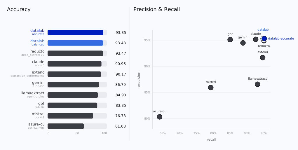
System	Mode	Accuracy	Precision	Recall	Coverage
datalab-accurate	accurate	93.85	95.32	95.11	620
datalab	balanced	93.48	95.30	94.79	620
reducto	deep_extract v2	93.47	94.91	95.02	620
claude	opus 5	90.96	95.17	92.60	575
extend	extraction_performance	90.17	91.67	94.66	620
gemini	3.7-flash	86.79	94.48	88.81	526
llamaextract	agentic_plus	84.93	86.57	93.13	616
gpt	5.6-sol	83.85	95.11	84.99	615
mistral	ocr 4.1	76.78	85.93	79.27	574
azure-cu	gpt-4.1-mini	61.08	80.32	64.07	569

Each mean is calculated over how many documents the provider could actually process — the coverage column. Short coverage is a limit of the provider: the document either exhausted its output limit, or its schema was rejected as too large.

We will continue to improve the tooling, auditability and fairness of this benchmark. We are keen to hear your thoughts (especially if you disagree). The scoring code is on GitHub and the data is on Hugging Face.

Data

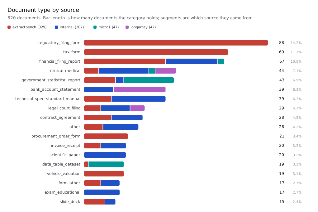
620 documents across 4 sources:

Source	# Documents	Coverage
extractbench	329	Forms, filings, decks.
internal	202	Dense scalar schemas, small documents.
micro1	47	Very large tables.
longarray	42	Large tables with repeated scalars.

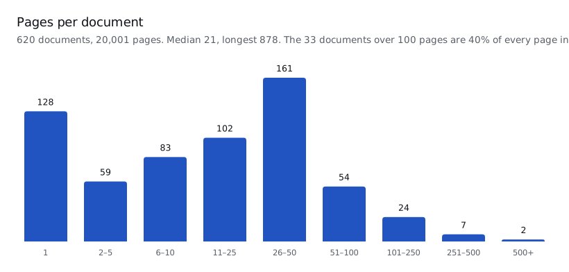
Here is a breakdown of the documents:

Scorer

Challenges of scoring

The challenge with extraction scoring is with ambiguous addresses of values. An address is a path to a scalar value that you walk along a dictionary to get to that value. For example, the single address of the following dictionary {"a": {"b": "c"}} is ("a", "b").

In lots of extraction tasks, we want to extract a variable number of JSON objects. The user specifies this with an "array" type in the JSON schema. This is often used for large tables — we want to extract many rows from a table that should respect a certain schema.

The issue here is that one small mistake could cost nearly an entire table’s worth in score when we score naively. For example, on a table with 100 rows, if the model misses the first row, each predicted row will be positionally off-by-one, leading to a terrible score even though the model effectively got 99/100 correct.

Our scorer

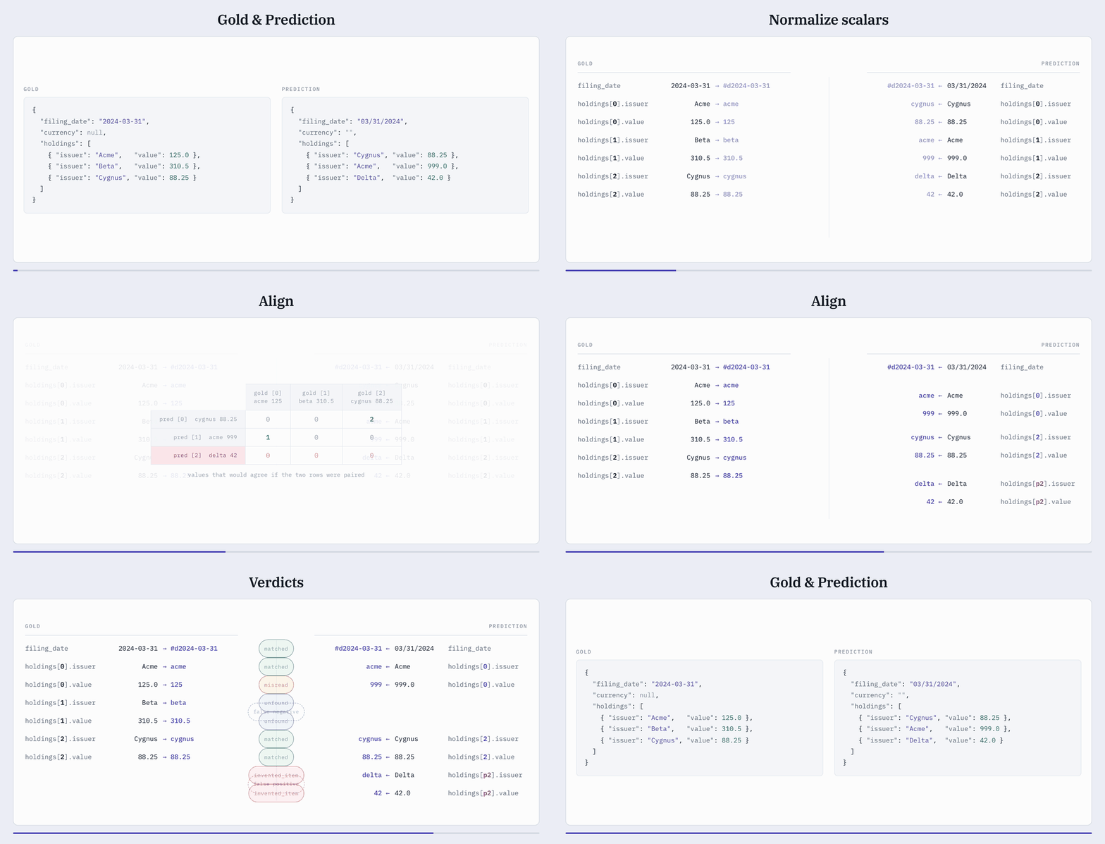
Our scorer is deterministic and has a simple design. It has three components:

• Document normalization;
• Scalar normalization; and
• Pairing leaf addresses:
  • If unambiguous, pair exactly; and
  • If ambiguous, Hungarian match based on content (recursively in case of nested arrays of objects).

And it works in the following stages:

1. Normalize document;
2. Flatten prediction and gold JSON dictionary to addresses mapped to their scalar values;
3. Normalize scalar values of the flattened addresses; and
4. For each array that appears, Hungarian match (recursively for nested arrays) based on array element content to align ambiguous predicted and gold addresses. There may be unmatched predicted addresses — false positives — and unmatched gold addresses — false negatives.

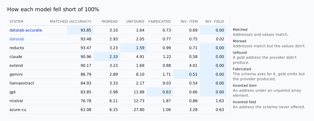
For each document, this process produces one Verdict per unique scalar address, aligned via Hungarian matching when needed. The options are:

• matched: was matched and the values match;
• misread: was matched and the values don’t match;
• unfound: ground truth has the address, prediction doesn’t;
• fabricated: schema offered the address, ground truth is silent but prediction exists;
• invented_item: an array element’s scalar prediction that paired with nothing; or
• invented_field: an address the schema never declared.

These are mutually exclusive in our code and also semantically. The one interesting judgement call we made here is that an address falls under invented_item if it falls within an unpaired item (i.e. row), even if the address was an invented field within that array element’s schema. We think this is the right call: it signals that this was counted against the model for inventing an item. Addresses outside of arrays that the schema never declared are invented_field.

How we handle nulls

One inconsistency across scoring harnesses is how they handle null. The challenge is how to know when a model is omitting something versus asserting something. This is the difference between saying a cell in a table doesn’t have a value versus the cell containing the text "n/a".

We handle nulls in the following way (for both ground truth and prediction):

• We flatten both JSONs to get a mapping from addresses to their values; and
• We inspect the value and ask if it states nothing (omission) or not (assertion):
  • "", None, "\t\n" all get turned to None; and
  • "NA", "-", "--" all remain.

For every address that has a None value after these steps, drop the entire address. This means that omitting an address is the same as having the address point to None. We think this is the right approach since, otherwise, the metric can be gamed via schema width.

The gaming would be as follows: add hundreds of optional fields to the ground-truth schema without them actually existing in the benchmark’s documents. The models then get awarded for finding nothing by getting (basically) free matches between None and None, arbitrarily inflating scores.

Metrics

All metric formulas are based on verdict count, which itself is an address count after alignment. The number of all verdicts is total.

shared = |matched|
       + |misread|

|gold| = |matched|
       + |misread|
       + |unfound|

|pred| = |matched|
       + |misread|
       + |fabricated|
       + |invented_item|
       + |invented_field|

total  = |matched|
       + |misread|
       + |unfound|
       + |fabricated|
       + |invented_item|
       + |invented_field|

The headline metrics are:

• accuracy → |matched| / total;
• recall → |matched| / |gold|; and
• precision → |matched| / |pred|.

The power of verdicts

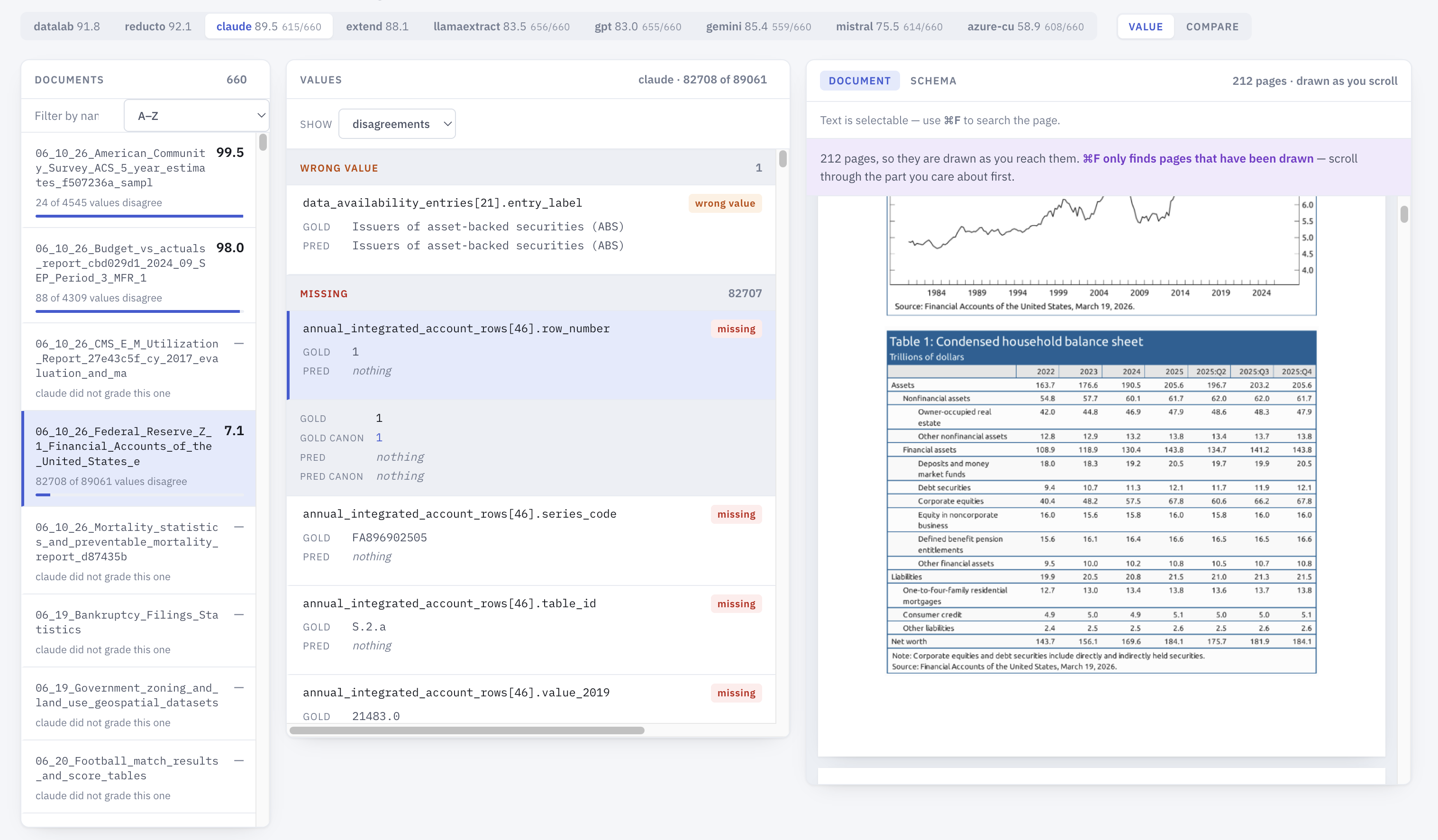
What the Verdicts allow us to do is provide auditability through results, versus just the code that led to those results. Metrics decompose into counts of Verdicts, so what you see at the top can be interrogated through a ladder of abstraction, which helps interpretability.

One thing we’re building is a small UI that breaks down results by Verdict and lets you cross-reference this alongside the PDF and schema. Here’s a preview:

What’s next

We look forward to receiving community feedback and continuing to refine the benchmark, add more tooling and build out OmniExtractBench further. In the coming weeks, we’ll talk more about some of the issues we see with other benchmarks. We’ll also launch tools to help you evaluate extraction results and build confidence.

As always, the benchmark that matters most is the one you run on your own documents — point our playground at your ugliest files and check our numbers against your own. If you have feedback on the benchmark, email us at [email protected].