 Talk to Sales
 Benchmarks
View scores and output across OCR models spanning many document categories.
Want to run these evals on your own documents?
Talk to Sales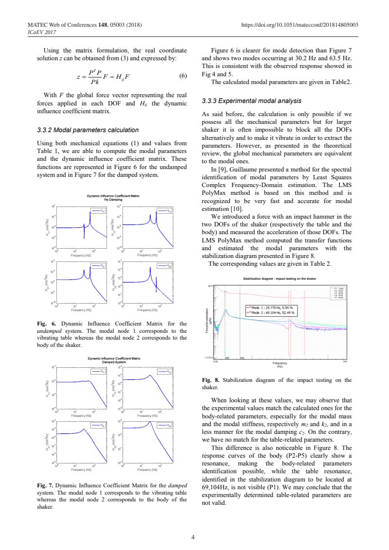
ICoEV 2017
https://doi.org/10.1051/matecconf/201814805003
Using the matrix formulation, the real coordinate solution can be obtained from (3) and expressed by:
With the global force vector representing the real forces applied in each DOF and the dynamic influence coefficient matrix.
3.3.2 Modal parameters calculation
Using both mechanical equations (1) and values from Table 1, we are able to compute the modal parameters and the dynamic influence coefficient matrix. These functions are represented in Figure 6 for the undamped system and in Figure 7 for the damped system.

Fig. 6. Dynamic Influence Coefficient Matrix for the undamped system. The modal node 1 corresponds to the vibrating table whereas the modal node 2 corresponds to the body of the shaker.

Fig. 7. Dynamic Influence Coefficient Matrix for the damped system. The modal node 1 corresponds to the vibrating table whereas the modal node 2 corresponds to the body of the shaker.
Figure 6 is clearer for mode detection than Figure 7 and shows two modes occurring at 30.2 Hz and 63.5 Hz. This is consistent with the observed response showed in Fig 4 and 5.
The calculated modal parameters are given in Table 2.
3.3.3 Experimental modal analysis
As said before, the calculation is only possible if we possess all the mechanical parameters but for larger shaker it is often impossible to block all the DOFs alternatively and to make it vibrate in order to extract the parameters. However, as presented in the theoretical review, the global mechanical parameters are equivalent to the modal ones.
In [9], Guillaume presented a method for the spectral identification of modal parameters by Least Squares Complex Frequency-Domain estimation. The LMS PolyMax method is based on this method and is recognized to be very fast and accurate for modal estimation [10].
We introduced a force with an impact hammer in the two DOFs of the shaker (respectively the table and the body) and measured the acceleration of those DOFs. The LMS PolyMax method computed the transfer functions and estimated the modal parameters with the stabilization diagram presented in Figure 8.
The corresponding values are given in Table 2.

Fig. 8. Stabilization diagram of the impact testing on the shaker.
When looking at these values, we may observe that the experimental values match the calculated ones for the body-related parameters, especially for the modal mass and the modal stiffness, respectively and , and in a less manner for the modal damping . On the contrary, we have no match for the table-related parameters.
This difference is also noticeable in Figure 8. The response curves of the body (P2-P5) clearly show a resonance, making the body-related parameters identification possible, while the table resonance, identified in the stabilization diagram to be located at 69,104Hz, is not visible (P1). We may conclude that the experimentally determined table-related parameters are not valid.
4